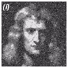
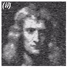
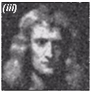
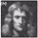
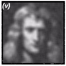
The results of the filtering processes are shown below. Figure (i) is the raw, unfiltered data. Figure (ii) the 1D averaged data and Figs. (iii)-(v) are 3x3, 5x5 and 7x7 filtered respectively. Note the loss of image definition as the order of the filter is increased.

When using this method of averaging or median filtering, a balance must be struck between the reduction of noise and the loss of definition. We will see in Lecture 7 how signals and waveforms may be broken down into Fourier components i.e. analysed in terms of the frequencies that contribute to the signal. Median filtering may be thought of as removing the high frequency components in the image (i.e. those components that are responsible for producing sharp changes in contrast in the image).